What is VLOOKUP?
VLOOKUP means Vertical Lookup.
It searches for a value in the first column of a table and returns related data from another column.
Step 1: Click the cell where you want the answer
Example: Click cell E2
Step 2: Type the formula
=VLOOKUP (102, A2:C4, 3,)
Step 3: Press Enter
Result will be: 90
What is HLOOKUP?
HLOOKUP means Horizontal Lookup.
It searches for a value in the first row of a table and returns related data from another row.
Example Data (Enter in Excel)
| A1 | B1 | C1 | D1 |
|---|---|---|---|
| ID | 101 | 102 | 103 |
| A2 | B2 | C2 | D2 |
|---|---|---|---|
| Name | Rahul | Priya | Amit |
| A3 | B3 | C3 | D3 |
|---|---|---|---|
| Marks | 85 | 90 | 78 |
Find the Marks of ID 102
Step 1: Click the cell where you want the result
Example: Click cell B5
Step 2: Type the formula
=HLOOKUP(102, A1:D3, 3, FALSE)
Step 3:Press Enter
Result:
You will get 90.
What is XLOOKUP?
XLOOKUP is the modern and better version of VLOOKUP & HLOOKUP.
It works vertically and horizontally both .
Example Data (Enter in Excel)
| A1 | B1 |
|---|---|
| ID | Name |
| A2 | B2 |
|---|---|
| 101 | Rahul |
| 102 | Priya |
| 103 | Ami |
Step 1:Click on empty cell (Example: D2)
Step 2:Type formula:
=XLOOKUP(102, A2:A4, B2:B4)
Step 3:Press Enter
Result:
You will get Priya
REFERENCE Formulas
These formulas refer to cell positions.
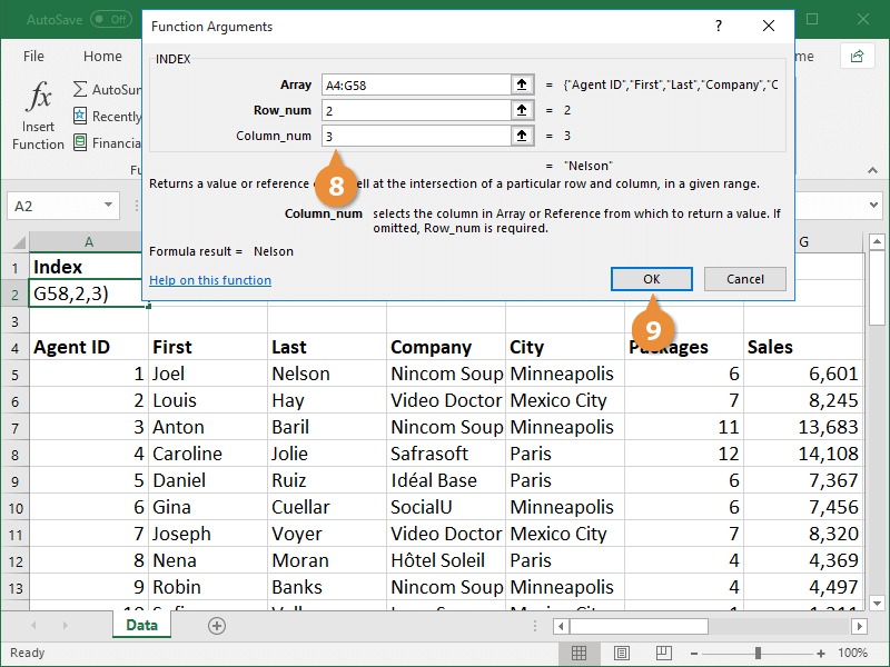
A) INDEX FORMULA
What INDEX Does:
Returns value from a specific position in a table.
SYNTAX
=INDEX(array, row_number, column_number)
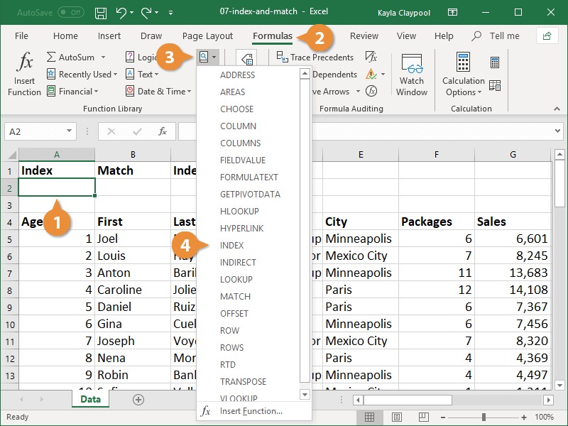
- Click in the cell where you want to add the INDEX function.
- Click the Formulas tab.
- Click the Lookup & Reference button in the Function Library group.
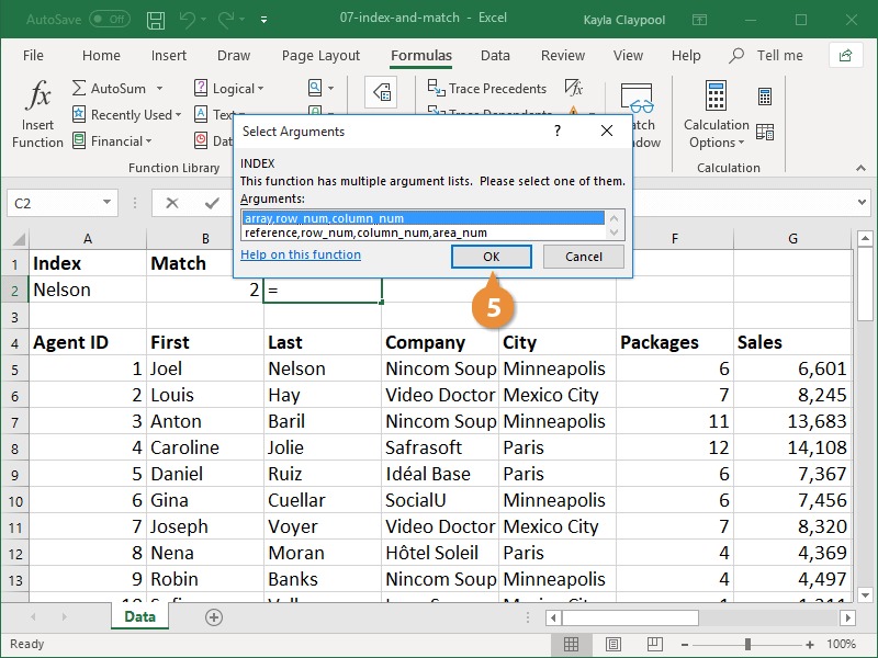
- Select INDEX.
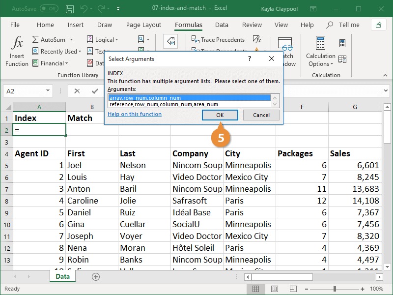
- Select the array argument and click OK.
- Enter the range of data you want to search in the Array field.
- Enter a new lookup value to search for in the first row of data.
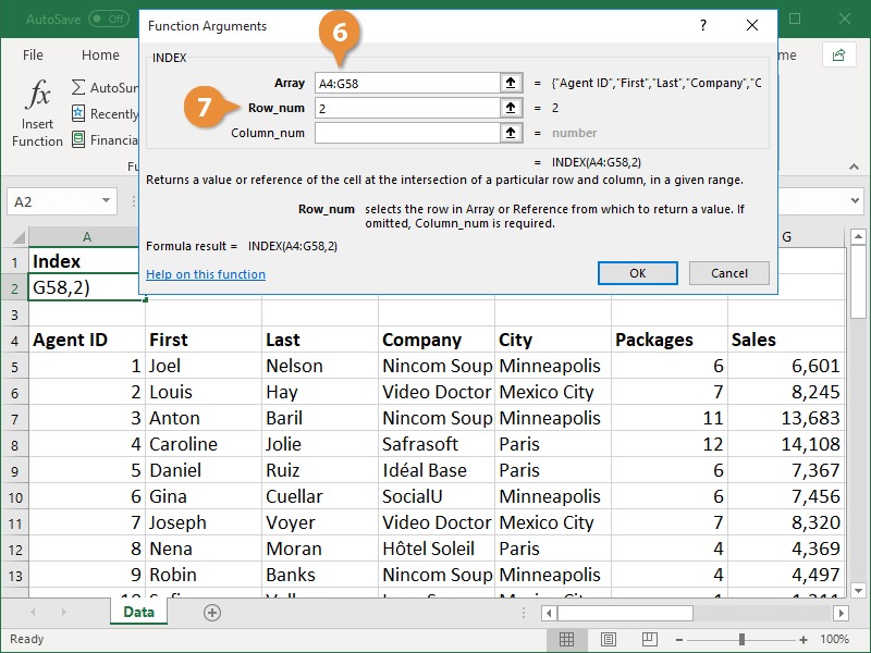
- Enter the row in the array you want search in the Row_num field.
- Click OK.
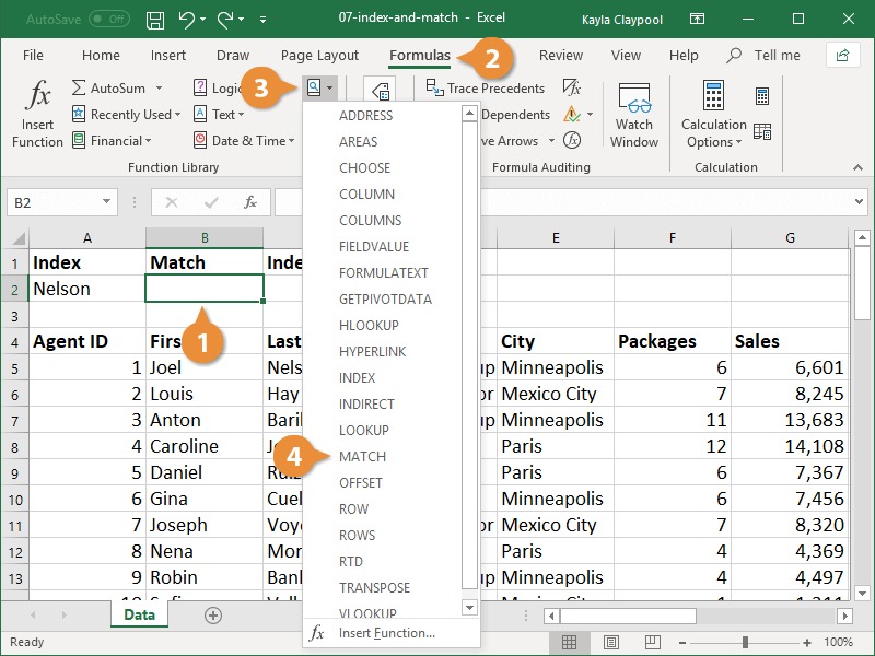
B)MATCH FORMULA
What MATCH Does:
Finds position of a value in a range
SYNTAX
=MATCH(lookup value, lookup array, 0)
- Click in the cell where you want to add the MATCH function.
- Click the Formulas tab.
- Click the Lookup & Reference button in the Function Library group.
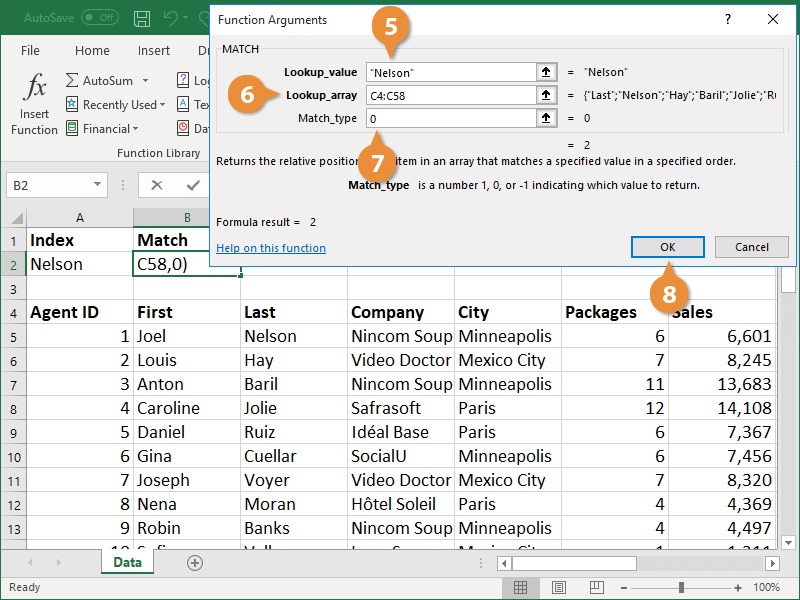
- Select MATCH.
- Enter the value you want to search for in the Lookup_value field.
- Enter the value you want to search for in the Lookup array field.
- Enter 0 in the Match_type field to search for an exact value.
- Click OK.
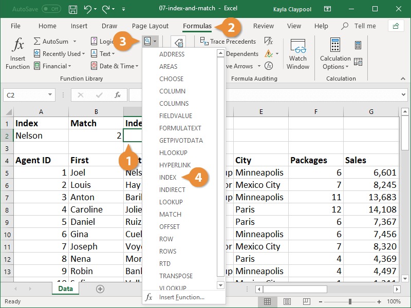
3) INDEX + MATCH FORMULA
When used together, the INDEX and MATCH functions combine to be a powerful force in Excel. After seeing how helpful these functions are, many people choose to use these instead of the VLOOKUP function.
- Click the cell where you want to add the nested functions.
- Click the Formulas tab.
- Click the Lookup & Reference button in the Function Library group.You will start with the INDEX function and nest the MATCH function within it.
- Select INDEX.
- Select the array argument option in the Select Arguments dialog box and click OK.
- Type the cell range you want to search within to locate a value.This is often a single column of data, not a multi-column range.
- Enter the MATCH function in the Row_num field to specify the lookup value.If the array is a single column, there is no need to add a value to the Column_num field, as there is only one column being searched.
- Click OK.