Excel Slicer

What is an Excel Slicer?

The slicer is a filtering tool that was introduced in Excel 2010. Unlike dropdown menus, it gives you interactive buttons to filter your PivotTables and tables. You can narrow down your data with a single click and the best part is, you’ll always know which filters are active.

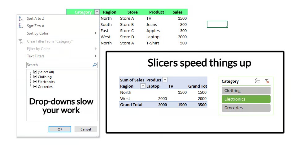
Most of the time, I use slicers to track my monthly projects and isolate specific categories in a report. Instead of running through dropdown menus, I just click a button and instantly see the data I need — it’s that simple.

Slicers help me focus on what’s important without getting distracted by everything else. That’s why, for me, the biggest win is how they cut through the noise. They’ve also become a go-to when I’m building dashboards because they add a polished and professional touch.

So, if you haven’t tried slicers yet, maybe try them now because they’re one of those tools that are as valuable for beginners as they are for experts.

How to Insert an Excel Slicer

Now that you know what slicers are, I will walk you through how to add them to your Excel tables, PivotTables, and PivotCharts. It’s super easy, and I’ll share a few tips as well to make the process even more effective.

Add slicers to a PivotTable 

Here’s how you can add a slicer to a PivotTable:

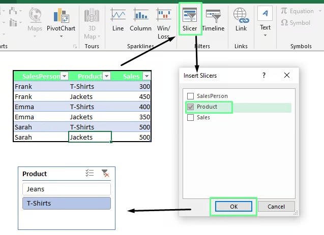
1. Click anywhere on your PivotTable.
2. Go to the Insert tab, find the Filters group, and click Slicer. Alternatively, you can head over to the Analyze tab and, under the Filter group, select Insert Slicer.
3. A window will pop up showing all the fields in your PivotTable. Check the boxes next to the ones you want to filter with a slicer.

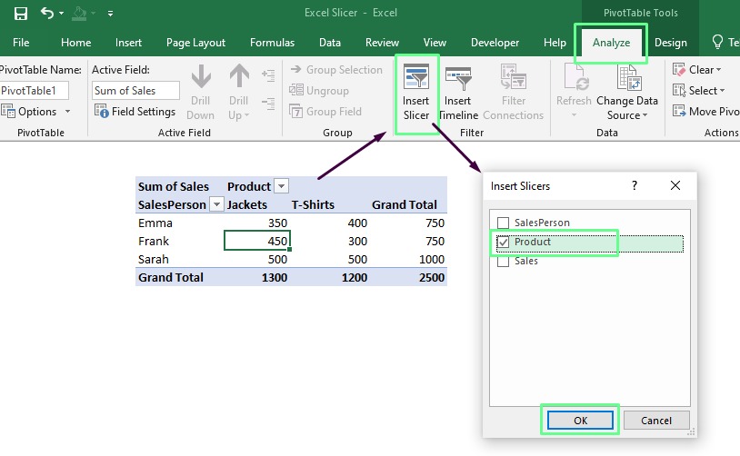
4. Click OK, and the slicer will appear on your sheet.

Add slicers to a PivotChart

Here’s how you can add a slicer to a Pivot chart.

1. Click anywhere on your PivotChart.
2. Go to the Analyze tab. From the Filter group, click Insert Slicer.
3. Check the fields you want to filter. Then, Click OK.

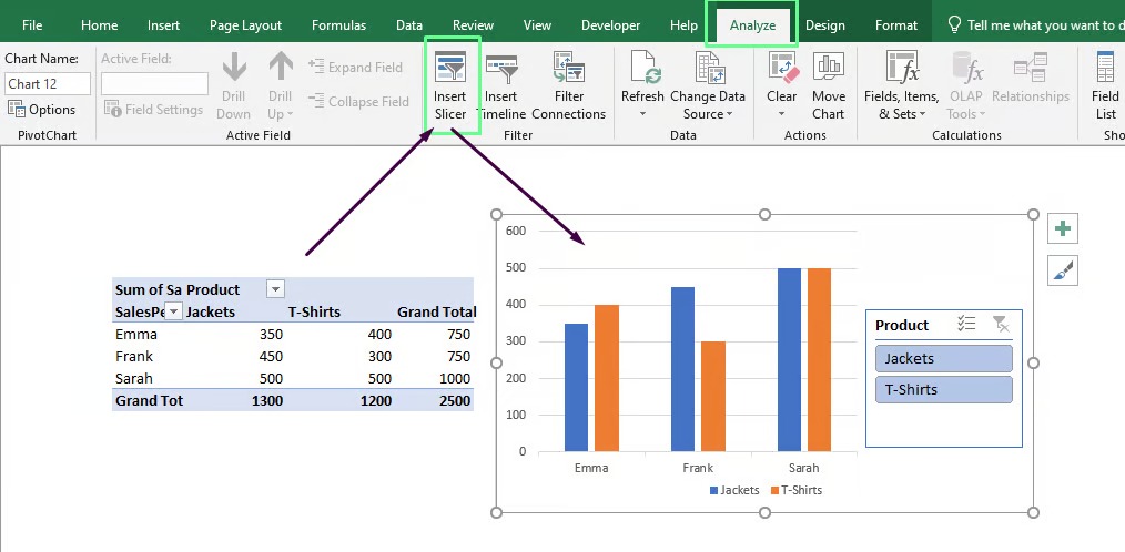
When I use slicers, I hide the chart’s filter buttons because they clutter the view. To clean things up, I even resize the chart area to fit the slicer inside. It keeps everything neat and easy to work with.

As a note, if your PivotTable and PivotChart are connected, the same slicer will work for both.

Add slicers to an Excel table

If you work with a regular table in Excel (and not PivotTables), slicers are still an option. Here’s how to add them:

1. Click anywhere inside your table.
2. Go to the Insert tab, find the Filters group, and click Slicer.
3. In the window that pops up, check the boxes for the columns you want to filter.
4. Click OK, and the slicer will appear and be ready to use.

When you choose fields for a slicer, think about what will make your data easier to handle. For example, slicing by fields like Region, Month, or Salesperson would work best if you analyse sales data. So, focus on the dimensions that matter most to your analysis to quickly find the important insights.

How to Customise the Excel Slicer Appearance

Let me show you how you can tweak your slicer appearance to match your workbook style.

Change the slicer style 

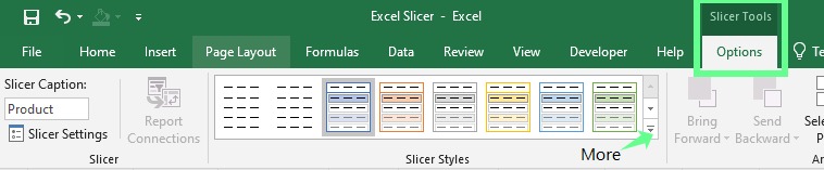
Click on your slicer to bring up the Slicer Tools tab. Under this tab, go to the Options section and check out the Slicer Styles group. Here, you’ll see several built-in styles — pick one you like.

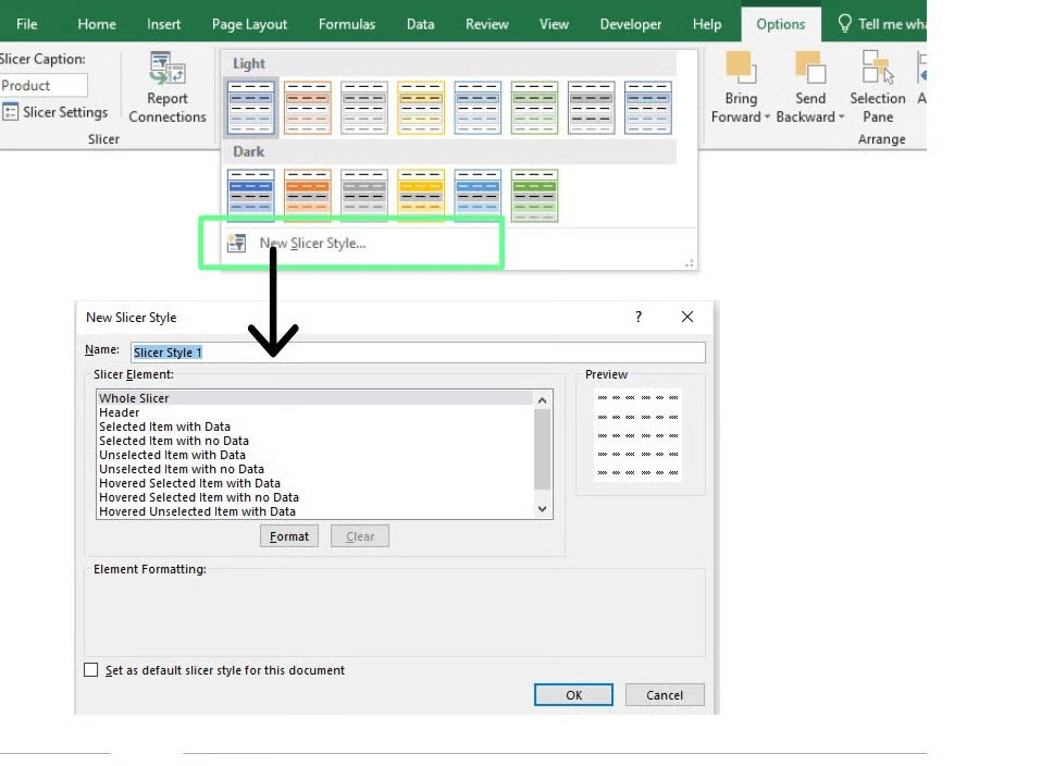
If you don’t like any of the built-in styles, you can create one. Click the drop-down (More) button and select New Slicer Style. From here, you can build a custom style that matches your spreadsheet theme.

For example, if I’m working with a dashboard that has a cool blue theme, I’ll create slicer colors in complementary shades of blue. It would make everything look more cohesive.

Adjust slicer settings

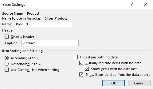
If you want to tweak your slicer further, right-click on it and select Slicer Settings. From here, you can make a lot of adjustments. For example, you can hide the slicer header if it doesn’t add value or hide items without data to make it look cleaner and more focused. 

Although these are minor adjustments, they can make the slicer much more user-friendly.

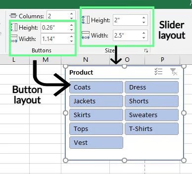
Optimize slicer layout 

When my slicer has a lot of items, the default single-column view drives me crazy because it requires so much scrolling. To fix that, I click the slicer, go to the Slicer Tools Options tab, and adjust the Columns setting. I usually set it to 2 or 3 columns, depending on the slicer content.

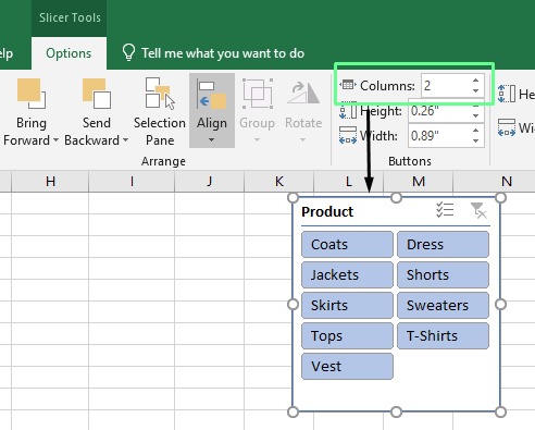
I also adjust the button sizes to make everything look balanced. To do so, go to the Slicer Tools Options tab, tweak the height and width settings, or drag the edges of the slicer until they look right. However, I’d recommend keeping the slicer buttons large enough to be easy to click but not so big that they take over the whole sheet. 

Advanced Excel Slicer Techniques

Besides basic filtering, you can create interactive reports and dashboards with Excel slicers. Let me show you some of my favourite tricks for doing that.

Connect slicers to multiple PivotTables

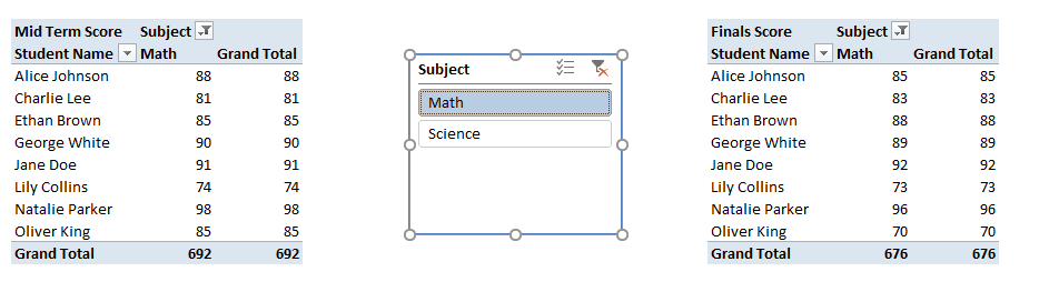
One of the coolest features of slicers is the ability to link a single slicer to multiple PivotTables. This is really helpful when you work with related datasets. It lets you filter all your data at once with a single click — you don’t have to update each table manually. Here’s how I used this technique to analyse student performance data: 

1. I created all the PivotTables I wanted to link. To keep things manageable, I placed them on the same worksheet.
2. Next, I gave each PivotTable a unique name. This made it much easier to identify them when I set up the connections.
3. Then, I added a slicer to one of the PivotTables.
4. Once the slicer was in place, I selected it, went to the Slicer Tools Options tab, and clicked Report Connections. Alternatively, you can right-click on the slicer and choose Report Connections.

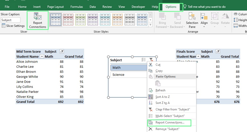
5.In the dialog box that popped up, I checked the boxes for the PivotTables I wanted to link to the slicer and clicked OK.

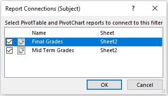
Now, I can filter this data with a single click to see the students’ midterm and final scores. It saves so much time and makes analysing multiple PivotTables easy. Making a connection this way also helps avoid unforced errors.

Optimize Excel slicer performance

Slicers can sometimes slow down or behave unexpectedly if you work with large datasets. When I started, I ran into a few common problems and had to figure out how to fix them. Here are those issues and the solutions that worked for me: 

• Slow performance: You may notice your slicers lag or respond slowly. This usually happens because they’re trying to process too much data. To fix this, filter out data you don’t need or create a summary table with only the important information. This will improve slicer performance and give you a smoother overall experience.
• Multiple slicers for multiple tables: Managing multiple slicers for different tables is messy and hard to track. Instead of creating separate slicers, connect one slicer to multiple tables using Report Connections. This keeps everything cleaner and easier to manage while maintaining consistency across your data.
• Clicking doesn’t filter anything: If your slicer isn’t filtering, it’s likely not linked to the correct tables. This can happen when the connections aren’t set up properly. To resolve this, right-click the slicer, select Report Connections, and make sure it’s connected to the tables you want to filter.
• Seeing old data in the slicer: Sometimes, slicers display items that no longer exist in your dataset. This happens when deleted items aren’t cleared from the slicer’s settings. To avoid this, go to Slicer Tools Options, then Slicer Settings, and uncheck Show items deleted from data source.
• Non-updated data: If the slicer isn’t reflecting the latest changes in your data, it may be because you haven’t refreshed the PivotTable. Right-click the PivotTable and select Refresh to update the slicer.
• Cluttered slicer layout: A default slicer layout with a single column or oversized buttons may require a lot of scrolling. To fix this, go to Slicer Tools Options, adjust the column count, and resize the slicer. 
• Hidden slicer: If you can’t see your slicer, it may have been accidentally moved behind other elements. Right-click it and choose Bring to Front to make it visible again.

Excel Slicer vs. PivotTable Filters

You might now be wondering what the difference is between an Excel slicer and a PivotTable filter. Let’s compare the key differences to see which option may be best for you.

Excel Slicer	PivotTable Filters
Simple and easy to use. Click the option you want, and the data updates instantly.	Uses a dropdown interface where you have to select and click through menus.
Can connect to multiple PivotTables and charts for more control over related datasets.	Tied to a single PivotTable, which limits its scope.
Movable and can be placed anywhere, even within a chart or dashboard layout.	Fixed within the table interface.
Offers a wide range of formatting, such as customizing headers, colors, and layout.	Limited customization options.
Easy to interpret at a glance, even with large datasets.	Can be harder to read and interpret if you work with a lot of data.
Takes up more space on the worksheet, especially with multiple slicers.	Compact and doesn’t take up additional space.

When to use each

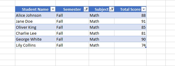
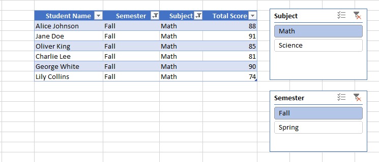
Let’s say I want to filter all students’ math grades for the fall semester. Now, I’ll do this using both filters and slicers to help you understand which option may suit you better. 

Using filters: I’d click the dropdown menus in the Semester and Subject columns to select Fall and Math. It gets the job done but can feel a bit clunky if I’m doing this repeatedly or sharing with others who aren’t Excel-savvy.

Using slicers: I’d insert slicers for Semester and Subject and place them right next to my table. With just two clicks, I can visually filter the data. The slicers also make it easier for others to interact with the report without extra instructions.

In short, filters are great for quick tasks where space matters. But slicers are more suitable when you need an interactive and user-friendly experience, especially on dashboards or with multiple PivotTables.