How to Use Conditional Formatting in MS Excel?
Conditional formatting is used to change the appearance of cells in a range based on your specified conditions.
The browser version of Excel provides a number of built-in conditions and appearances:
Conditional Formatting Example
Here, the Speed values of each Pokémon is formatted with a Colour Scale:
Colour Scale Formatting Example
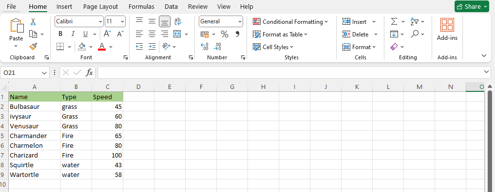
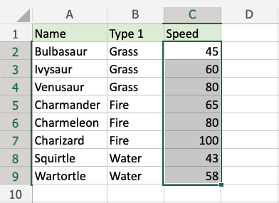
Highlight the Speed values of each Pokémon with Colour scale conditional formatting.
Conditional formatting, step by step:
1.Select the range of Speed values C2:C9
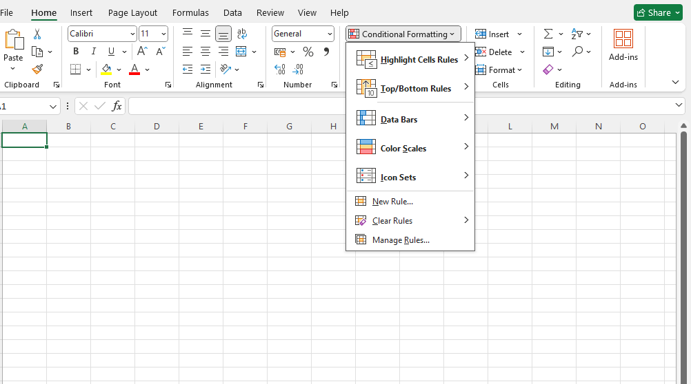
2.Click on the Conditional Formatting icon ![]() in the ribbon, from the Home menu.
in the ribbon, from the Home menu.
3.Select Colour Scales from the drop-down menu.
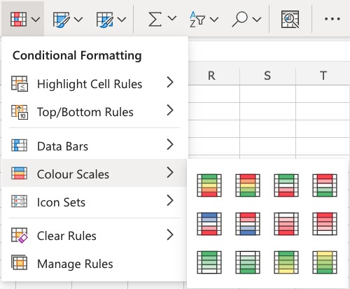
There are 12 Colour Scale options with different colour variations.
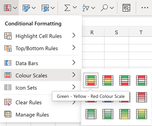
The color on the top of the icon will apply to the highest values.
4.Click on the “Green – Yellow – Red Colour Scale” icon.
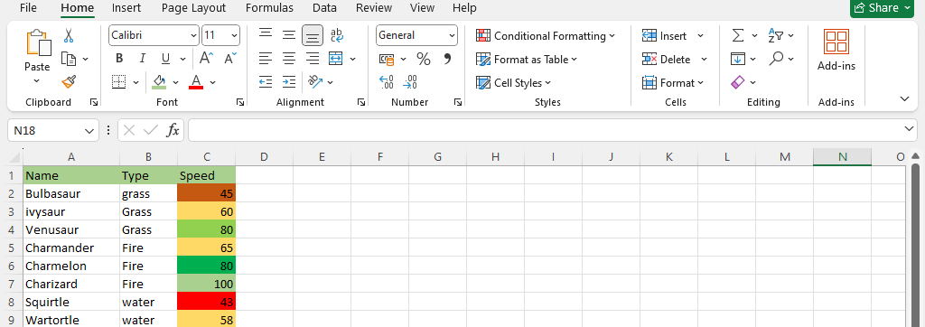
Now, the Speed value cells will have a colored background highlighting:
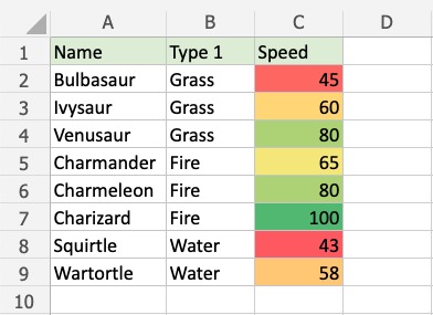
Dark green is used for the highest values, and dark red for the lowest values.
Charizard has the highest Speed value (100) and Squirtle has the lowest Speed value (43).
All the cells in the range gradually change color from green, yellow, orange, then red.