Data Bars
Data Bars are premade types of conditional formatting in Excel used to add colored bars to cells in a range to indicate how large the cell values are compared to the other values.
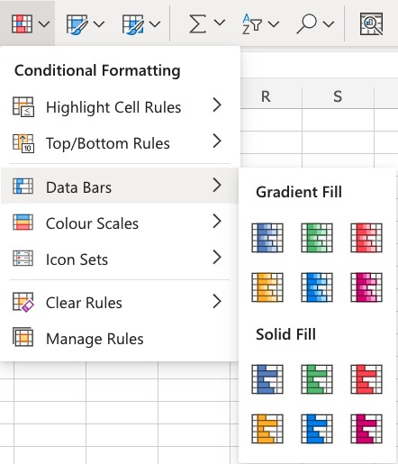
Here is the Data Bars part of the conditional formatting menu:
Data Bars Example
You can choose any range for where the Highlight Cell Rule should apply. It can be a few cells, a single column, a single row, or a combination of multiple cells, rows and columns.
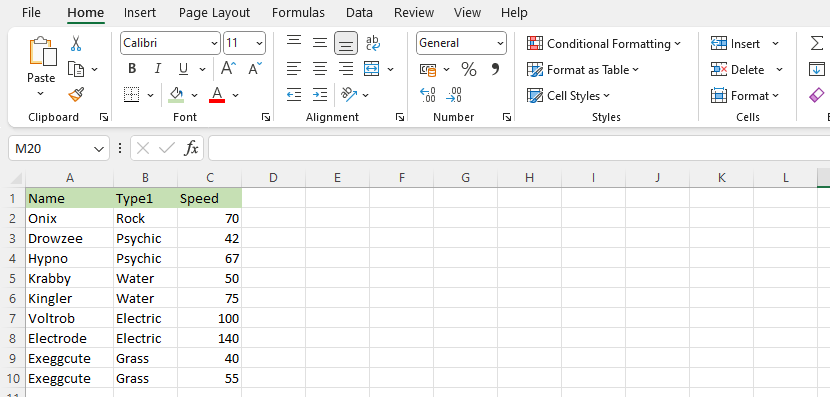
Let’s apply the Data Bars conditional formatting to the Speed values.
“Data Bars”, step by step:
1.Select the range C2:C10 for Speed values.

- Click on the Conditional Formatting icon
 in the ribbon, from Home menu
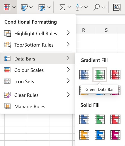
 - Select Data Bars from the drop-down menu
- Select the “Green Data Bars” color option from the Gradient Fill menu
Now, all of the Speed value cells have a green bar showing how big the value is compared to the other values in the range:
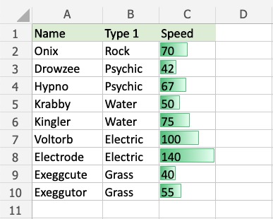
Electrode has the highest value, 140, so the bar fills the entire cell.
The other bars are scaled relative to the highest value and 0 by default.
Exeggcute has the lowest value, 40, so this is the shortest bar. Though, it is larger than 0, so there is still a small bar.
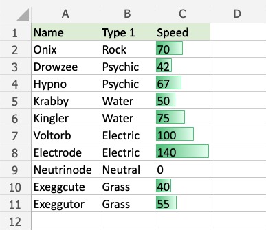
Let’s see what happens if we add a fictional Pokémon with a 0 Speed value:

The fictional Neutrinode has a Speed value of 0, so this becomes an invisible “minimum” bar.
Let’s see what happens if we add another fictional Pokémon with a negative Speed value:
Now, the fictional Positroid has the lowest Speed value, -140, so this becomes an invisible “minimum” bar.
Neutrinode’s Speed value of 0 is now in the middle between -140 and 140, so the cell has a bar filling half the cell.
Electrode still has the highest Speed value, 140, so this bar still fills the entire cell.